Your k is a decision, and the model will not tell you that you made it
Somebody hands you a number. It is called k, it came out of a calibration, and it is going to decide where you post your quotes. Whoever hands it to you says it was fitted to the data (a phrase which, in my experience, does most of its work by sounding like a measurement when what it describes is a choice).
We fitted it to the data too. Twice, on the same three days of coinbase BTC-USD, with the same code (nothing changed between the two runs except which stretch of the curve we let the estimator see). The first time k came out between 0.79 and 1.20 (that is the spread across the three days, which is itself worth noticing). The second time it came out between 5.23 and 6.79.
That is not a small disagreement. Out of the model comes an optimal half-spread of $1.12 in the first case and $0.15 in the second (that is the first day; across the three, the far window runs $0.83 to $1.26 against $0.15 to $0.19 near the touch, and the gap never closes); one of them tells you to stand a dollar away from the mid and the other tells you to stand fifteen cents away, which are not two versions of the same strategy but two different businesses, and the data have no opinion about which one you are in.
Where a calibrated k comes from, and why nobody checks it
The whole of it is smaller than its reputation, so here it is. The model is Avellaneda and Stoikov's, from 2008. The machinery needs to know how quickly your chance of being filled falls off as you move away from the middle of the market, and it assumes that the fall-off is exponential (convenient, which is why it was assumed):
δ is how far your quote sits from the mid, in dollars. λ is how often somebody comes and takes it, in trades per second. A is how often that would happen if you stood right at the middle, where nobody actually stands. And k is the whole question: how fast the interest dies as you back away from it.
Two things about k are worth knowing before anybody quotes you one.
The first is that 1/k is a distance rather than a coefficient. It is the step you have to take before the flow thins out by a factor of e, which is to say by about two thirds. A k near 1 describes a market where interest is spread over roughly a dollar; a k near 6 describes one where it is spread over about seventeen cents. Different worlds, same formula, and the formula holds no opinion about which one you are standing in. It reads that off k, and only off k.
The second is how k reaches your quotes. Put the inventory term aside (k does not appear in it) and what the model instructs you to do is
where γ is how much you dislike risk. For any γ small next to k, that expression is 1/k to within a fraction of a per cent. Which means the number somebody handed you is not an input that feeds your quoting distance through some chain of reasoning where errors might dilute. It very nearly is your quoting distance, wearing a Greek letter.
Everything else the model asks for is yours: how much risk you tolerate, how long your horizon runs, how much you hate carrying inventory overnight. You can be wrong about those in the way a person is wrong about their own preferences, which is to say not very. k is the only input on which you can be wrong about the world, confidently, with a decimal point.
So we went and looked at the curve.
The arrival curve is not a curve. It is three things stacked together
A quote sitting half a tick from the mid sees fifty-eight per cent of all print flow (that is the first of the three days; the other two give sixty-two and fifty-seven, and I stay with the first from here on so that the numbers come from one day). Move it half a tick further out, to a full tick, and thirty-four per cent is left. A quarter of everything that trades in a day fits inside that single half-tick. That is not the beginning of a decay; it is a spike sitting on top of the origin (a queue effect, most likely, though we have not taken that apart), and whatever it is, it belongs to a different phenomenon than the one the model spends its equations describing.
Then, across the first ten cents, essentially nothing happens. The arrival rate goes from 3.97 trades per second to 3.55, an eleven per cent decline while the distance grows by a factor of ten. (Under the assumed exponential, a tenfold increase in distance should flatten you. It doesn't.) This region, and here is the whole difficulty in one sentence, is exactly where a market maker stands all day, which means the assumption at the centre of the model is false in precisely the place where the model is being used to make decisions.
And only past the plateau does the curve finally start bending the way the theory wants. The third region is the one of the three that the model describes correctly, and it is also the one you are not standing in. The exponential works exactly where you have no use for it.
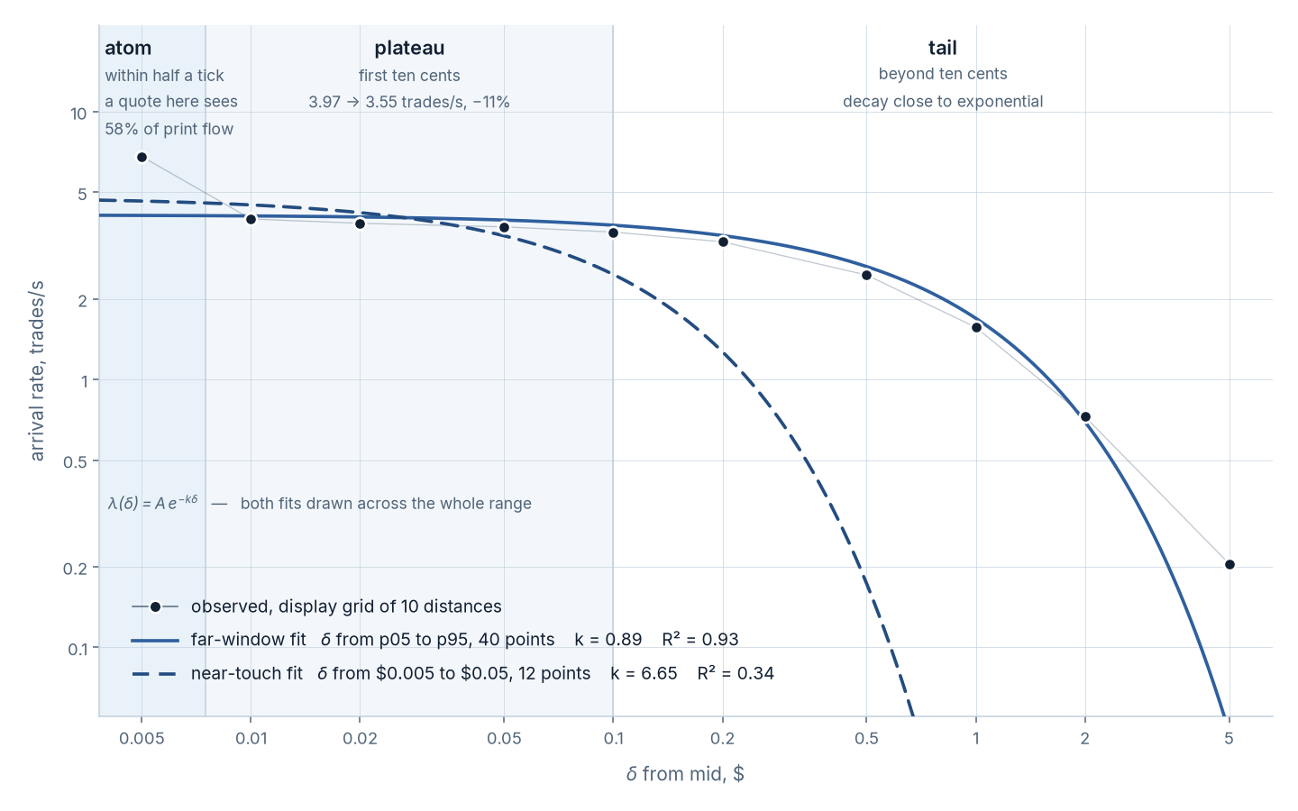
One exponential; three regions; a choice.
The comfortable part, which is the dangerous part
Here is the mechanism that lets this survive review, and it is worth understanding because it generalises far beyond market making.
There are three regions, and you pick one window. Then you fit, then you compute R2, and R2 is computed inside the window you picked. It is a grade awarded by the examiner who also wrote the exam and chose the room. The far fit scores 0.93 – on all three days, to two decimals – and looks excellent. The near fit lands between 0.32 and 0.35 (twelve points, close to the touch) and looks like noisy data in need of cleaning.
Neither number knows that the other window exists.
| Fitting window | k | R2 | What it says |
|---|---|---|---|
| Far window | 0.79–1.20 | 0.93 | Excellent fit where nobody posts a quote |
| Near touch | 5.23–6.79 | 0.32–0.35 | The region where quotes actually stand |
The same k fitted on the same three days under two windows. The gap between windows exceeds the spread between days.
And the obvious way to settle it (take the higher R2) is precisely wrong, which is the sort of thing that happens when a statistic gets used as a substitute for looking. That 0.93 is real. It is earned on the far stretch of the book, out where the fit is easy and where nobody posts a quote. The near one is real too, and what it is telling you, in the only language it has, is that the exponential does not describe this market where the market actually is.
You are being rewarded for measuring in the place where measurement is convenient. This is not a market-making problem. It is the standard failure mode of anyone who calibrates anything.
More data will not save you
When two estimates disagree the reflex is to want more data; three days feels thin, and three months feels rigorous.
It isn't, and the reason is worth stating precisely: an estimation problem has a true value underneath it, and your measurements scatter around that value, so more of them tighten the scatter. Here there is no value underneath. The model demands one exponential and the market supplied three regions. Run it on a year and you get the same two answers with narrower confidence intervals, which is to say the same disagreement stated with more authority.
More data makes a misspecified model more convincing, not less. That is the part people miss.
What I would ask, and what I would not accept
If somebody shows you a calibrated k (yours, a vendor's, a paper's, the one underneath a backtest) the question is not what the value is. Ask instead which stretch of the curve it came from, and why that stretch.
If the answer is a shrug, or "the standard range", or the number arrives without a window at all, you are not looking at a measurement. You are looking at somebody's decision wearing a lab coat. A backtest that does not name its fitting window is not reproducible, no matter how careful everything around it appears; and appearing careful, in this business, is cheap.
None of this makes the model useless. It is fine at what it does, which is to convert assumptions into quotes, and it does that faithfully and fast. It simply cannot tell you that one of the assumptions you fed it was not true, because it was never designed to; you have to do that part yourself, by looking at the curve, which takes an afternoon and which almost nobody does.
In the pieces that follow I will show how we do it instead: on the same three days, without asking one exponential to describe three regions. It is not difficult. It is merely not what gets handed around.
Where I could be wrong
I would rather say it myself than have it said to me.
- This is one venue and one pair, coinbase BTC-USD, over three days in July 2026. I have not looked at other periods, other instruments, or other asset classes, and the failure of the exponential is established here, not everywhere.
- Every
matchprint is counted as its own event, so a marketable order that the exchange chops into several prints is counted several times, which inflates the rate further out. I have not measured what merging them does. - δ is measured against the mid of the preceding book snapshot, reconstructed to depth five, and whatever that reconstruction gets wrong, these numbers inherit.
- Both fits are ordinary least squares on the log of the intensity, over a 40-point grid far out and 12 points near the touch. A different estimator might behave differently; I have not tried one.
The maxim, then, and it costs nothing to apply.
Before you accept a calibrated number, ask which stretch of the world it was fitted to. If the answer does not exist, neither does the calibration.
Questions people ask about calibrating k
What is k in the Avellaneda–Stoikov model?
It is the decay rate of the fill intensity function λ(δ) = A e−kδ. Its reciprocal 1/k is a distance, the step you move away from the mid before order flow thins by a factor of e. A k near 1 describes a market where interest is spread over about a dollar; a k near 6, over about seventeen cents.
How is k calibrated in practice?
By fitting an exponential to the empirical arrival intensity measured against distance from the mid, usually by least squares on the log intensity. The result depends on which stretch of the curve is included, because the empirical curve is not a single exponential.
Why does the fitting window change the value of k?
Because the arrival curve on BTC-USD has three regimes. A spike at the origin, where a quote half a tick from the mid still sees 58 per cent of prints and a full tick out only 34, a plateau across the first ten cents where intensity falls only 11 per cent, and a decaying tail beyond it. Fitting the far range gives k between 0.79 and 1.20; fitting near the touch gives 5.23 to 6.79.
Does more data fix an unstable k?
No. More data narrows the confidence interval around each of the two answers without choosing between them, because the disagreement comes from model misspecification rather than sampling noise.
We do this kind of measurement
for funds and prop desks
Calibration audits, microstructure research and production engineering for low-latency trading systems.
Provenance
All figures come from our own measurement on coinbase BTC-USD trade prints against L3-reconstructed books, 1–3 July 2026, depth five. Values quoted here match the source measurement line for line: k of 0.79 to 1.20 and 5.23 to 6.79, R2 of 0.93 and 0.32, half-spreads of $1.12 and $0.15, 58 per cent of prints reaching half a tick or beyond, 3.97 falling to 3.55 trades per second across the first ten cents, an 11 per cent decline, 40 and 12 grid points, γ = 0.01.
The rhetorical devices in this piece (the figure who hands you a number, R2 compared to an exam, the closing maxim) carry no claims of their own. No personal anecdotes appear that did not happen. One work is cited, the paper whose assumption this piece tests. Every measurement reported here is our own, and where we have not measured something it is said so above.